Investment Portfolio Data Modeling
Interested in learning more about Cassandra data modeling by example? This example demonstrates how to create a data model for investment accounts or portfolios. It covers a conceptual data model, application workflow, logical data model, physical data model, and final CQL schema and query design.

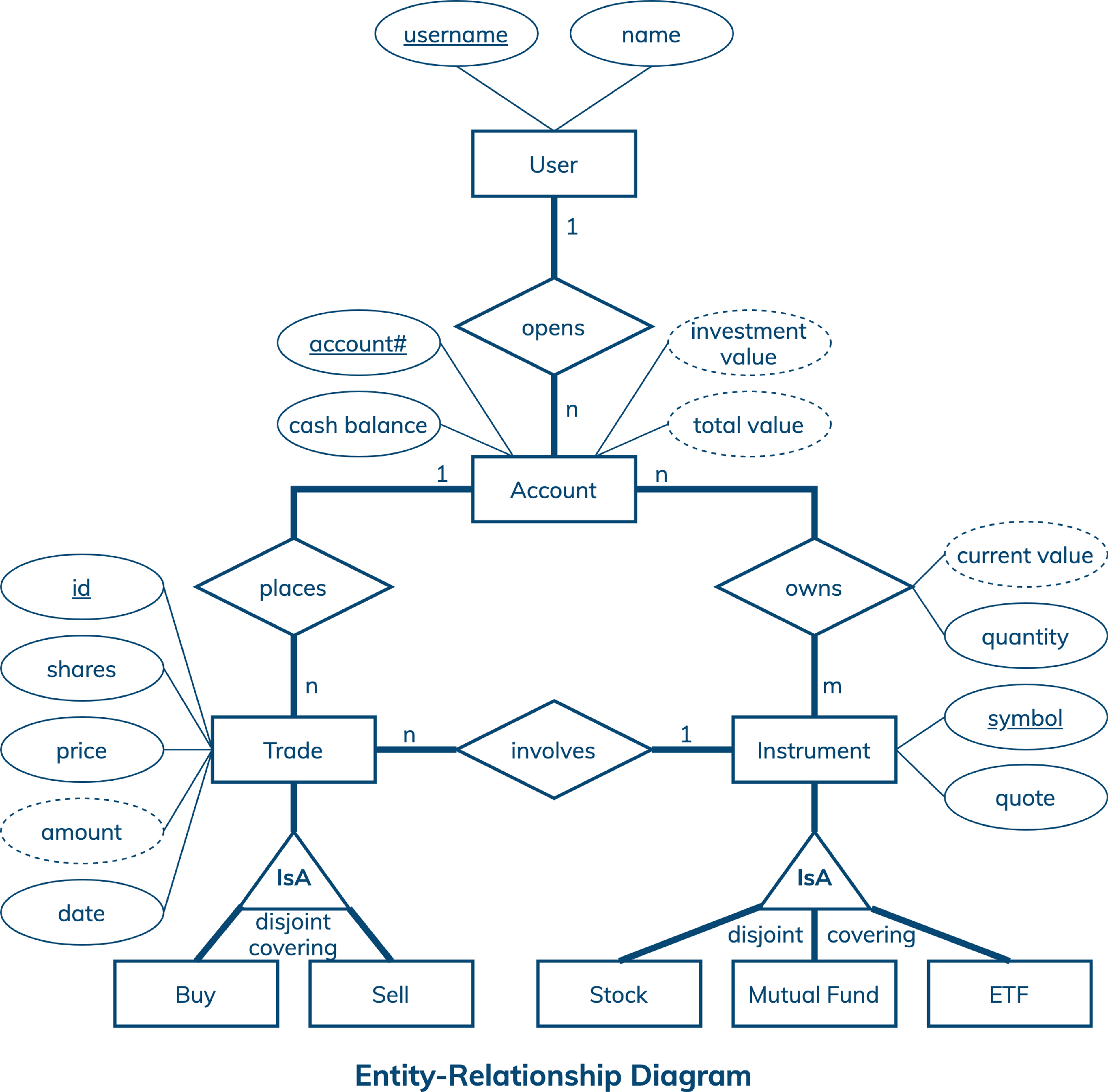
Conceptual Data Model
A conceptual data model is designed with the goal of understanding data in a particular domain. In this example, the model is captured using an Entity-Relationship Diagram (ERD) that documents entity types, relationship types, attribute types, and cardinality and key constraints.
The conceptual data model for investment portfolio data features users, accounts, trades and instruments. A user has a unique username and may have other attributes like name. An account has a unique number, cash balance, investment value and total value. A trade is uniquely identified by an id and can be either a buy transaction or a sell transaction. Other trade attribute types include a trade date, number of shares, price per share and total amount. An instrument has a unique symbol and a current quote. Stocks, mutual funds and exchange-traded funds (ETFs) are all types of instruments supported in this example. While a user can open many accounts, each account must belong to exactly one user. Similarly, an account can place many trades and an instrument can participate in many trades, but a trade is always associated with only one account and one instrument. Finally, an account may have many positions and an instrument can be owned by many accounts. Each position in a particular account is described by an instrument symbol, quantity and current value.
Note that the diagram has four derived attribute types, namely investment value, total value, current value and amount. Derived attribute values are computed based on other attribute values. For example, a current position value is computed by multiplying a quantity by a quote for a particular instrument. An account investment value is the sum of all current position values. And an account total value is the sum of a cash balance and an investment value. Last but not least, a trade amount is the product of a price and a number of shares. In general, while some derived attribute values can be stored in a database, others can be dynamically computed by an application.
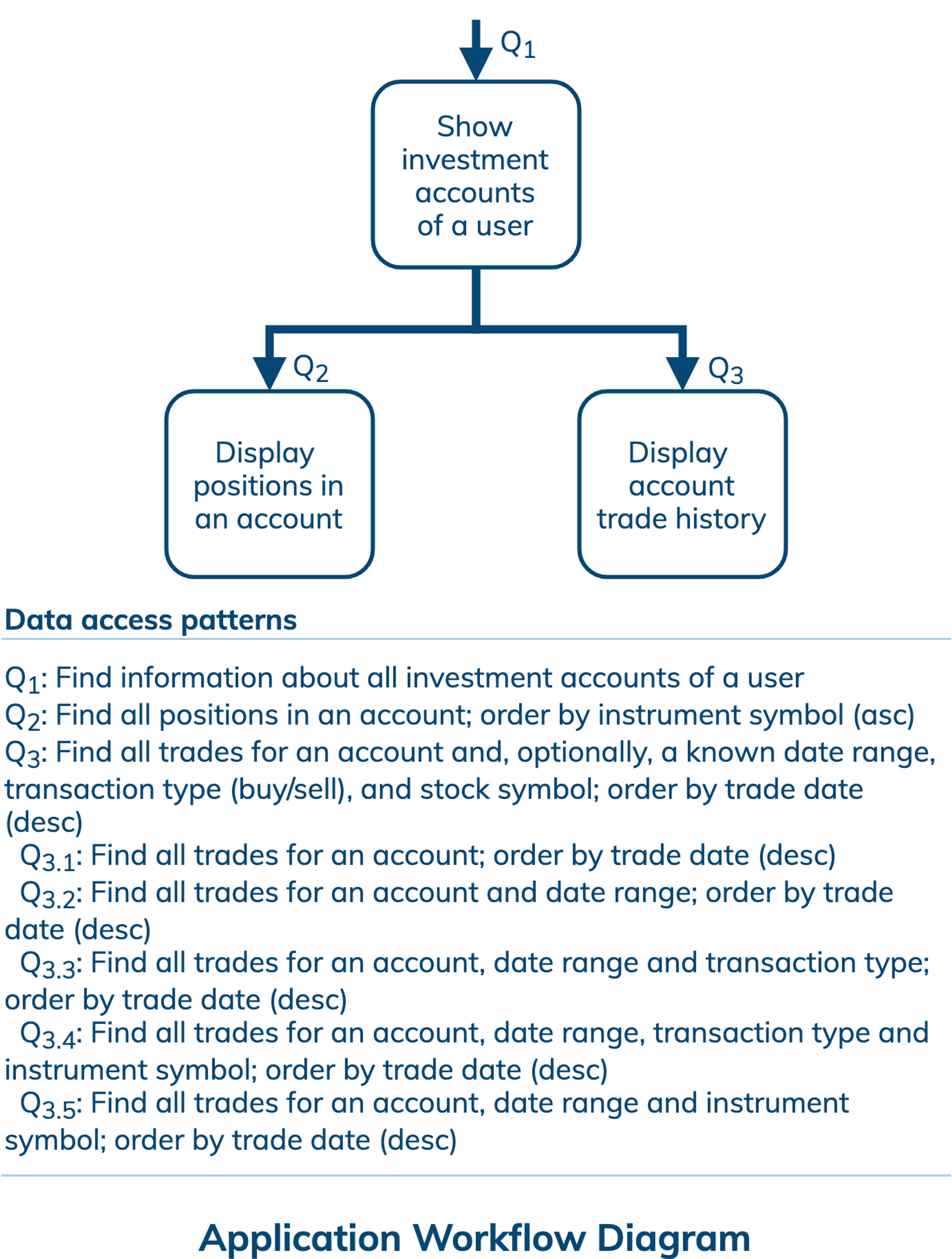
Application Workflow
An application workflow is designed with the goal of understanding data access patterns for a data-driven application. Its visual representation consists of application tasks, dependencies among tasks, and data access patterns. Ideally, each data access pattern should specify what attributes to search for, search on, order by, or do aggregation on.
The application workflow has an entry-point task that shows all investment accounts of a user. This task requires data access pattern Q1 as shown on the diagram. Next, an application can either display current positions in a selected account, which requires data access pattern Q2, or display information about trade history for a selected account, which requires data access pattern Q3. Furthermore, Q3 is broken down into five more manageable data access patterns Q3.1, Q3.2, Q3.3, Q3.4 and Q3.5. All in all, there are seven data access patterns for a database to support.


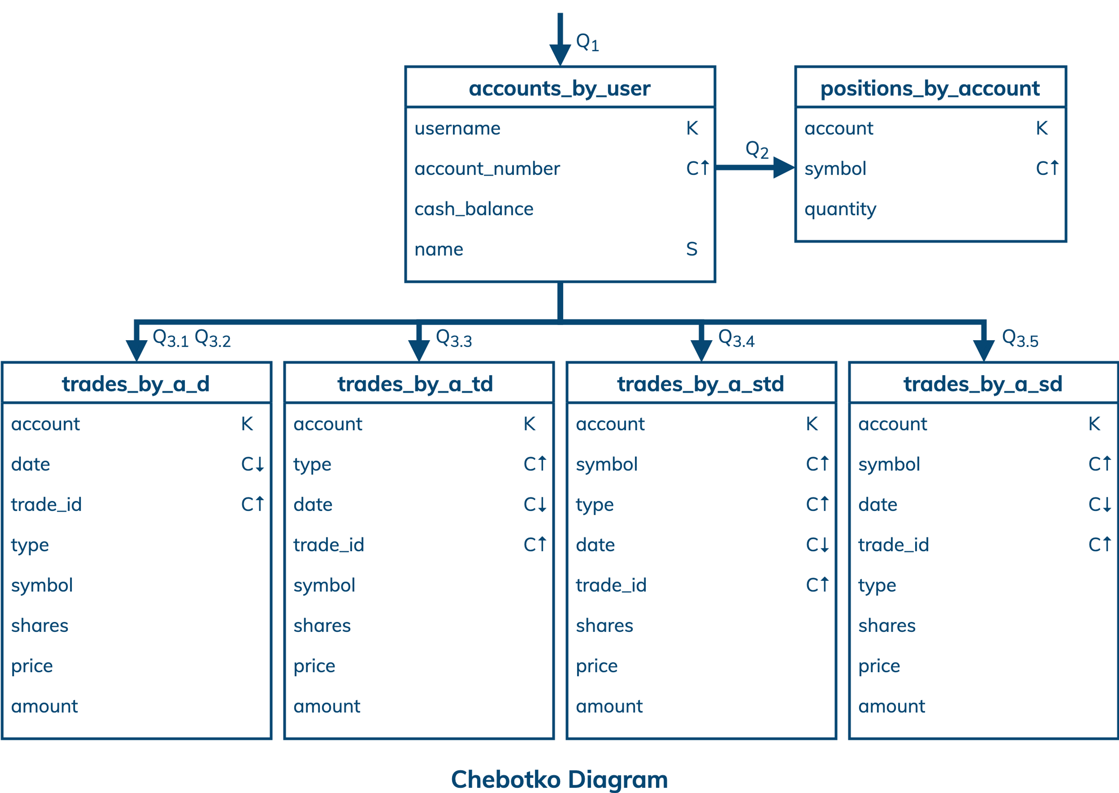
Logical Data Model
A logical data model results from a conceptual data model by organizing data into Cassandra-specific data structures based on data access patterns identified by an application workflow. Logical data models can be conveniently captured and visualized using Chebotko Diagrams that can feature tables, materialized views, indexes and so forth.
The logical data model for investment portfolio data is represented by the shown Chebotko Diagram. There are six tables that are designed to support seven data access patterns. All the tables have compound primary keys, consisting of partition and clustering keys, and therefore can store multiple rows per partition. Table accounts_by_user is designed to have one partition per user, where each row in a partition corresponds to a user account. Column name is a static column as it describes a user who is uniquely identified by the table partition key. Table positions_by_account is designed to efficiently support Q2. All positions in a particular account can be retrieved from one partition with multiple rows. Next, tables trades_by_a_d, trades_by_a_td, trades_by_a_std and trades_by_a_sd store the same data about trade transactions, but they organize rows differently and support different data access patterns. All four tables have the same partition keys, which represent account numbers, and are designed to retrieve and present trades in the descending order of their dates. Table trades_by_a_d supports two data access patterns Q3.1 and Q3.2, which are used to retrieve either all trades for a given account or only trades in a particular date range for a given account. Table trades_by_a_td also enables restricting a transaction type as in Q3.3. Furthermore, table trades_by_a_std supports querying using both an instrument symbol and transaction type as in Q3.4. Finally, table trades_by_a_sd supports Q3.5, which retrieves trades based on an account, instrument symbol and date range.
Note that not all information from the conceptual data model got transferred to the logical data model. Out of the four derived attribute types, only a trade amount will be stored in a database. Once a trade is completed, its amount is immutable and it makes sense to store it. In contrast, current position values, account investment values and account total values change frequently and it is better to compute them dynamically in an application. Also, the logical data model does not contain a catalog of all available instruments and their current quotes because this information is readily available from third-party systems.
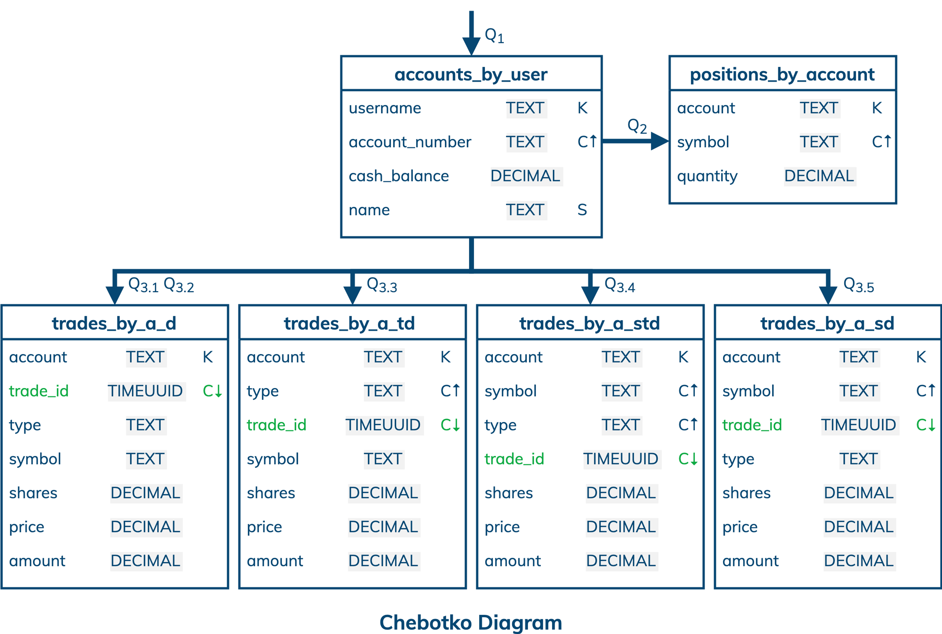
Physical Data Model
A physical data model is directly derived from a logical data model by analyzing and optimizing for performance. The most common type of analysis is identifying potentially large partitions. Some common optimization techniques include splitting and merging partitions, data indexing, data aggregation and concurrent data access optimizations.
The physical data model for investment portfolio data is visualized using the Chebotko Diagram. This time, all table columns have associated data types. Assuming the use case does not cover robo-advisors and algorithmic trading, it should be evident that none of the tables will have very large partitions. Any given user will at most have a few accounts. An account will normally have at most dozens of positions and possibly hundreds or thousands of trades over its lifetime. The only optimization applied to this physical data model is the elimination of columns with the name date in the four trade tables. Since trade ids are defined as TIMEUUIDs, trades are ordered and can be queried based on the time components of TIMEUUIDs. Date values are also easy to extract from TIMEUUIDs. As a result, storing dates explicitly becomes unnecessary. Our final blueprint is ready to be instantiated in Cassandra.

Skill Building
Want to get some hands-on experience? Give our interactive lab a try! You can do it all from your browser, it only takes a few minutes and you don’t have to install anything.
More Resources
Review the Cassandra data modeling process with these videos